Product Quantization
PQ并不是一种索引,而是创建复合索引中的一种Fine quantizer。
Introduction
向量相似性搜索可能需要大量内存,随着数据集大小的不断增加,内存占用会变得难以承受。PQ可以大幅压缩高维向量,甚至能减少97%的内存占用。(But at what cost?)
Quantization & Dimensionality-reduction
量化与降维不同,降维的目的是得到一个低维向量,而量化的目的是得到一个低精度向量。
tip
比如我有一个128维的FP32向量,我可以将其降维到64维(不是简单的裁切,比如使用PCA主成分分析),也可以将其量化为INT8向量。毫无疑问这两种方法都减少了向量的占用,而且都损失了信息。
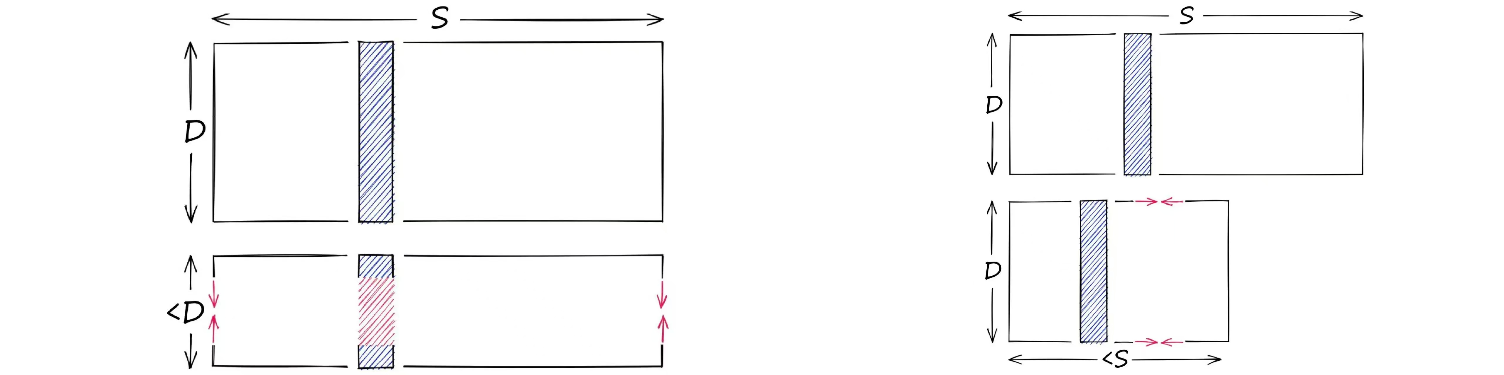 降维缩小了向量的维度,量化缩小了能表示的范围。
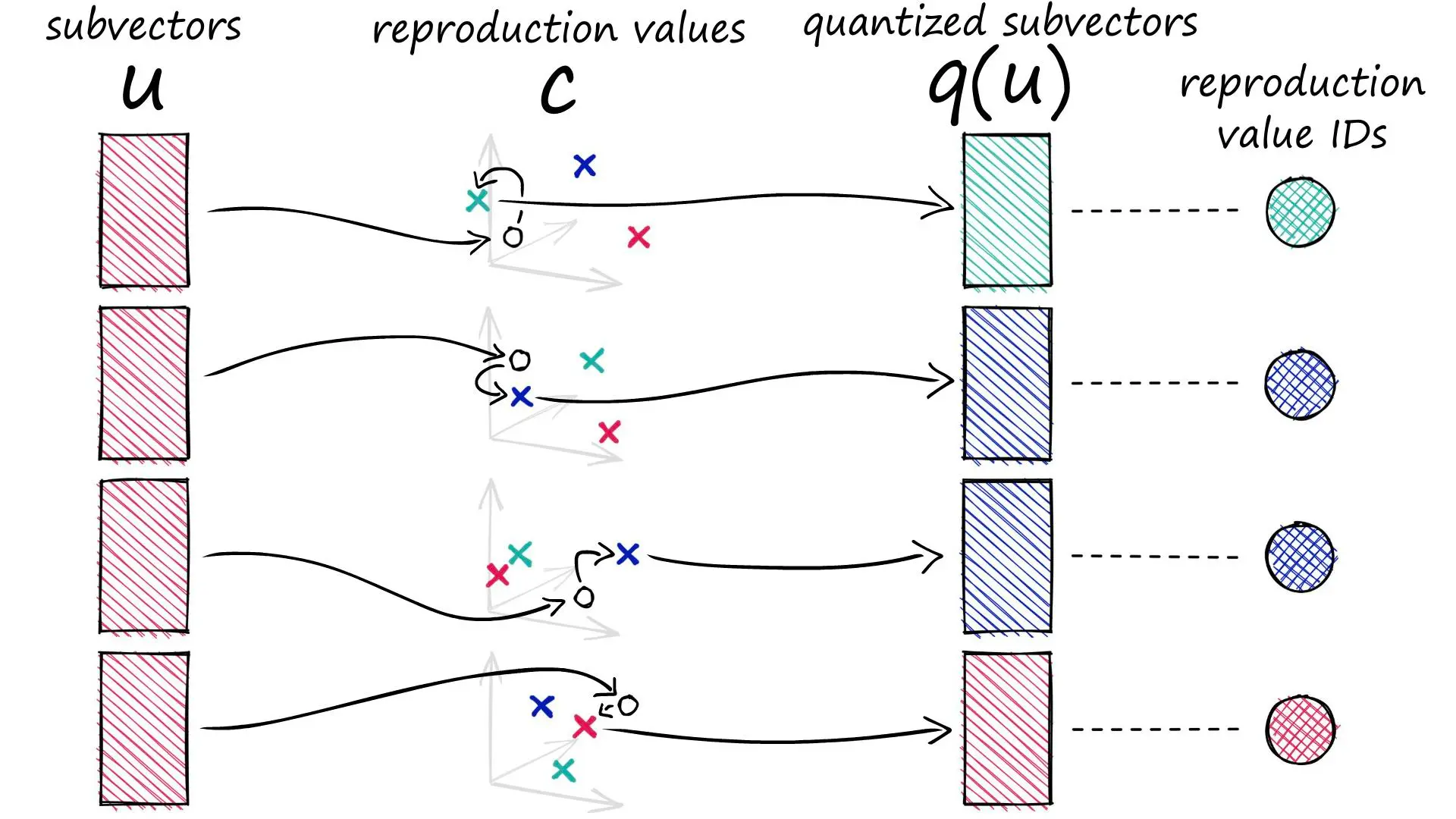
但是PQ并不是简单的将每个维度的信息量化成更低精度的表示。粗略地说,PQ先将向量分成几个子向量,每个子向量用它们所在的簇的ID来表示。
降维缩小了向量的维度,量化缩小了能表示的范围。
但是PQ并不是简单的将每个维度的信息量化成更低精度的表示。粗略地说,PQ先将向量分成几个子向量,每个子向量用它们所在的簇的ID来表示。
How PQ works
- 我有一些128维的向量。
- 按32维切分成4个子向量。
- 对所有128维向量的相同位置上的32维子向量进行聚类,例如得到128个簇。
- 用每个子向量所在簇的ID来表示这个子向量。(这样我们就能用2字节表示一个子向量)
- 最终128维的向量可以用8字节表示。
切分向量
x = [1, 8, 3, 9, 1, 2, 9, 4, 5, 4, 6, 2]

m = 4
D = len(x)
# ensure D is divisable by m
assert D % m == 0
# length of each subvector will be D / m (D* in notation)
D_ = int(D / m)

# now create the subvectors
u = [x[row:row+D_] for row in range(0, D, D_)]
print(u)
创建聚类 为方便起见,这里随机生成聚类中心。 再现值(reproduction values):用表示第个子向量的第个所选质心。
k = 2**5
assert k % m == 0
k_ = int(k/m)
print(f"{k=}, {k_=}")

from random import randint

c = []  # our overall list of reproduction values
for j in range(m):
    # each j represents a subvector (and therefore subquantizer) position
    c_j = []
    for i in range(k_):
        # each i represents a cluster/reproduction value position *inside* each subspace j
        c_ji = [randint(0, 9) for _ in range(D_)]
        c_j.append(c_ji)  # add cluster centroid to subspace list
    # add subspace list of centroids to overall list
    c.append(c_j)
定义函数计算L2距离和寻找最近邻居
`ids`记录距离每个子向量最近的质心的标识符。
def euclidean(v, u):
    distance = sum((x - y) ** 2 for x, y in zip(v, u)) ** .5
    return distance

def nearest(c_j, u_j):
    distance = 9e9
    for i in range(k_):
        new_dist = euclidean(c_j[i], u_j)
        if new_dist < distance:
            nearest_idx = i
            distance = new_dist
    return nearest_idx

ids = []
for j in range(m):
    i = nearest(c[j], u[j])
    ids.append(i)
print(ids)
q是用质心坐标表示的向量。
q = []
for j in range(m):
    c_ji = c[j][ids[j]]
    q.extend(c_ji)

print(q)
Example
Example
假设:
u = [[1, 8, 3], [9, 1, 2], [9, 4, 5], [4, 6, 2]]
我们有 m=4 个子空间,每个 u[j] 都有 k_=8 个可选的簇心 c[j]。
代码执行 nearest(c[j], u[j]),找到 u[j] 在 c[j] 里的最近簇心:
ids = [7, 1, 5, 3]
这意味着:
u[0] = [1, 8, 3]在c[0]里最接近c[0][7]u[1] = [9, 1, 2]在c[1]里最接近c[1][1]u[2] = [9, 4, 5]在c[2]里最接近c[2][5]u[3] = [4, 6, 2]在c[3]里最接近c[3][3]
然后 q 通过 ids 找到这些簇心,并拼接:
q = []
for j in range(m):
    c_ji = c[j][ids[j]]  # 取出最近的簇心
    q.extend(c_ji)       # 展开并拼接
最终:
q = c[0][7] + c[1][1] + c[2][5] + c[3][3]
Success
Success
x = [1, 8, 3, 9, 1, 2, 9, 4, 5, 4, 6, 2]

m = 4
D = len(x)
# ensure D is divisable by m
assert D % m == 0
# length of each subvector will be D / m (D* in notation)
D_ = int(D / m)

# now create the subvectors
u = [x[row:row+D_] for row in range(0, D, D_)]
print(u)

k = 2**5
assert k % m == 0
k_ = int(k/m)
print(f"{k=}, {k_=}")

from random import randint

c = []  # our overall list of reproduction values
for j in range(m):
    # each j represents a subvector (and therefore subquantizer) position
    c_j = []
    for i in range(k_):
        # each i represents a cluster/reproduction value position *inside* each subspace j
        c_ji = [randint(0, 9) for _ in range(D_)]
        c_j.append(c_ji)  # add cluster centroid to subspace list
    # add subspace list of centroids to overall list
    c.append(c_j)

def euclidean(v, u):
    distance = sum((x - y) ** 2 for x, y in zip(v, u)) ** .5
    return distance

def nearest(c_j, u_j):
    distance = 9e9
    for i in range(k_):
        new_dist = euclidean(c_j[i], u_j)
        if new_dist < distance:
            nearest_idx = i
            distance = new_dist
    return nearest_idx

ids = []
for j in range(m):
    i = nearest(c[j], u[j])
    ids.append(i)
print(ids)

q = []
for j in range(m):
    c_ji = c[j][ids[j]]
    q.extend(c_ji)

print(q)
Implementation in Faiss
在开始之前,我们需要获取数据。我们将使用 Sift1M 数据集。
import shutil
import urllib.request as request
from contextlib import closing

# first we download the Sift1M dataset
with closing(request.urlopen('ftp://ftp.irisa.fr/local/texmex/corpus/sift.tar.gz')) as r:
    with open('sift.tar.gz', 'wb') as f:
        shutil.copyfileobj(r, f)

import tarfile

# the download leaves us with a tar.gz file, we unzip it
tar = tarfile.open('sift.tar.gz', "r:gz")
tar.extractall()

import numpy as np

# now define a function to read the fvecs file format of Sift1M dataset
def read_fvecs(fp):
    a = np.fromfile(fp, dtype='int32')
    d = a[0]
    return a.reshape(-1, d + 1)[:, 1:].copy().view('float32')

# data we will search through
wb = read_fvecs('./sift/sift_base.fvecs')  # 1M samples
# also get some query vectors to search with
xq = read_fvecs('./sift/sift_query.fvecs')
# take just one query (there are many in sift_learn.fvecs)
xq = xq[0].reshape(1, xq.shape[1])

xq.shape # (1, 128)

wb.shape # (1000000, 128)
IndexPQ
import faiss

D = xb.shape[1]
m = 8
assert D % m == 0
nbits = 8  # number of bits per subquantizer, k* = 2**nbits
index = faiss.IndexPQ(D, m, nbits)
索引需要3个参数:
D:向量的维度m:子向量的数量nbits:每个子向量的位数
tip
nbits 定义了每个子量化器可以使用的位数,例如 nbits 为 11,每个子空间有2048质心。
因为使用的是使用聚类的 PQ,所以必须预先训练我们的索引。(这里直接使用 xb 进行训练),然后再将向量添加到索引中进行搜索
index.is_trained # False
index.train(xb)  # PQ training can take some time when using large nbits
index.is_trained # True
index.add(xb)

dist, I = index.search(xq, k) # 在dist中返回距离,在I中返回索引。

%%timeit
index.search(xq, k) # 1.49 ms ± 49.1 µs per loop (mean ± std. dev. of 7 runs, 1000 loops each)
使用L2索引作为基准,计算召回率
l2_index = faiss.IndexFlatL2(D)
l2_index.add(xb)

%%time
l2_dist, l2_I = l2_index.search(xq, k) # CPU times: user 46.1 ms, sys: 15.1 ms, total: 61.2 ms, Wall time: 15 ms

sum([1 for i in I[0] if i in l2_I]) # 50
搜索表现部分将放在Comparison中讨论。
IndexIVFPQ
为了进一步加快搜索时间,我们可以添加另一个步骤——使用 IVF 索引,它将减少搜索中比较的向量。
首先初始化IVFPQ索引:
vecs = faiss.IndexFlatL2(D)

nlist = 2048  # how many Voronoi cells (must be >= k* which is 2**nbits)
nbits = 8  # when using IVF+PQ, higher nbits values are not supported
index = faiss.IndexIVFPQ(vecs, D, nlist, m, nbits)
训练,添加,搜索...
index.train(xb)
index.add(xb)
dist, I = index.search(xq, k)
%%timeit
index.search(xq, k) # 86.3 µs ± 15 µs per loop (mean ± std. dev. of 7 runs, 10000 loops each)
sum([1 for i in I[0] if i in l2_I]) # 34
搜索速度从1.49ms降低到86.3µs,但是召回率从50%降低到34%。在给定等效参数的情况下,IndexPQ 和 IndexIVFPQ 都应该能够获得相同的召回率性能。
在这种情况下,提高召回率的办法是提高nprobe参数。(当nprobe=nlist时,IndexIVFPQ退化为IndexPQ)
| nprobe | 召回率 | 时延 |
|---|---|---|
| 1 | 34 | 86.3µs |
| 2 | 39 | |
| 48 | 50 | |
| 2048 | 50 | 1.49ms |
Conclusion
| Index | 高召回 | 低时延 | 低内存 |
|---|---|---|---|
| Flat | 🟢🟢🟢🟢🟢 | 🔴 | 🔴 |
| PQ | 🟡🟡🟡🟡 | 🟡🟡🟡 | 🟢🟢🟢🟢🟢 |
| IVFPQ | 🟡🟡🟡🟡 | 🟢🟢🟢🟢🟢 | 🟡🟡🟡🟡 |